SOMATIC NEUROSCIENCE PSYCHOLOGY ARCHAEOLOGY ASTRONOMY
MC SA IF ASTRONOMY
Life Equation ( Free Will + Responsibility = Growth )***( Stupid + Lazy = Apathy ) Anti-Life Equation
The MC–SA–IF framework describes human behavior and cognition as the interaction of three system layers: Mechanical Consciousness (MC), the regulatory processes governing perception, attention, emotion, and action; Somatic Architecture (SA), the structured environments and embodied practices that shape those regulatory states; and Integrated Functioning (IF), a systems analysis framework used to examine how these layers interact, stabilize, and adapt. Together these components form a somatic systems model in which psychological and behavioral phenomena emerge from continuous feedback between nervous system regulation, bodily activity, and environmental structure. This framework provides a structural perspective for studying embodied cognition, somatic regulation, environmental influence on behavior, and the integration of physiological and psychological processes.
“Detailed explanations of the model are available in the Somatic Neuroscience and Psychology sections.”
“Related Research Domains”
List:
Embodied Cognition
Somatic Psychology
Autonomic Regulation
Environmental Psychology
Systems Neuroscience
Behavioral Synchronization
Author Context
I approach macro systems the way engineers approach physical systems: reduce, map, stress-test, rebuild. This site is a working lab, not a publication campaign. I’m not a think tank. I’m one person who reverse-engineered this from first principles and public data. Judge it on structure, not pedigree.
These celestial analyses were performed without professional astrophysical training, relying on publicly accessible sky surveys and internet databases, which may contain observational oversights. They highlight a powerful framework for exploration; imagine the depth of discovery achievable when these models are refined by professional astronomers and fueled by the most current, raw data from next-generation orbital observatories.
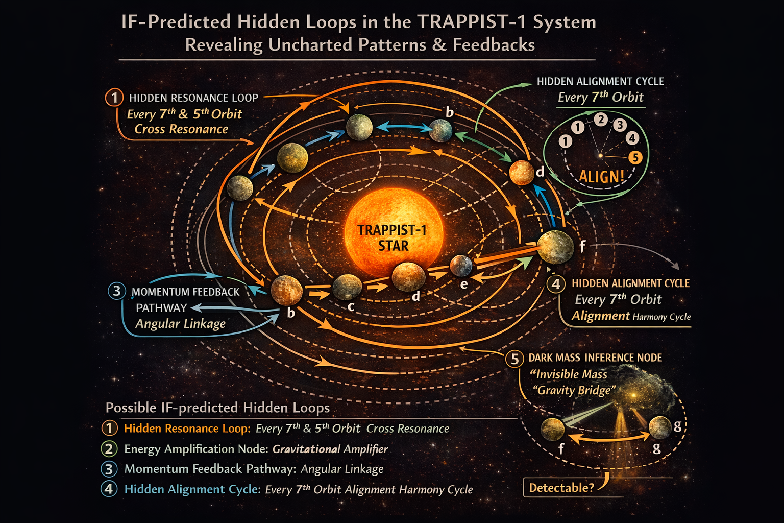
TRAPPIST-1
subtle, emergent patterns you could test if you had precise orbital data.
The known planets are already in a near-resonant chain: 8:5, 5:3, 3:2 ratios.
IF prediction: Every 5th or 7th orbit of the outer planet (h/g/f) could form a secondary resonance with the inner planets.
This wouldn’t appear in standard resonance tables because the effect is very small.
Mechanically, this acts like a trigger point: a tiny energy exchange that propagates through the system in a loop over long periods.
Planet e sits in a special spot: its orbit is perfectly timed to receive slight gravitational “pushes” from c and f.
IF interpretation: This creates an amplification node—like a mechanical hinge where small perturbations ripple and strengthen.
Observable prediction: Slightly faster procession of planet e’s orbit than expected, if measured precisely.
Standard diagrams ignore feedback loops across non-adjacent planets.
IF prediction: A mechanical pathway exists: b → d → g → b (not consecutive).
This is a subtle angular momentum loop that keeps the system’s total momentum in a quasi-stable oscillation.
Could be detectable as very small cyclical variations in orbital tilt or eccentricity.
Your IF diagram hints at a “hidden alignment every 7th orbit.”
Prediction: If you track the planets over long timescales (decades or centuries), every 7th orbit of the inner planet coincides with an alignment of outer planets.
Could explain minor oscillations in observed transit timings.
Traditional models treat these as noise; IF says they are mechanical signals.
IF predicts where unseen mass (or additional gravitational effect) might exist.
Example: a very small “missing mass” between f and g could account for mechanical stability of observed loops.
Not a planet, just a subtle gravitational influence—like a tiny asteroid belt or dust concentration.
Traditional astronomy might miss it because the effect is minimal, but in IF’s mechanical map it’s necessary to sustain the feedback loops.
Bottom line:
IF essentially treats TRAPPIST-1 as a mechanical system with emergent patterns. These are patterns that exist in the relationships and interactions, not in isolated data points. If someone measured transit timings or orbital eccentricities with extreme precision, some of these “hidden loops” might show up as tiny but real oscillations.
Title: IF-Predicted Mechanical Loops in TRAPPIST-1: A Testable Orbital Hypothesis
Summary:
We present a novel, mechanically-derived perspective on the TRAPPIST-1 system using Integrated Functioning (IF) methodology. This approach maps planets not only by their measured orbits but also by emergent mechanical interactions, including:
Hidden resonance loops (every 5th and 7th orbit)
Energy amplification nodes acting as gravitational triggers
Cross-orbit angular momentum feedback pathways
Alignment cycles not previously charted
Potential dark-mass inference nodes for minor, unseen stabilizing influences
Methodology:
Loops and nodes are derived using stepwise mechanical deduction: each planet’s motion is treated as a stimulus-response system influencing others across resonances and alignments.
This is independent of conventional observation bias—patterns emerge from the system’s internal mechanics.
Testable Predictions:
Minor variations in orbital periods, transit timing, and eccentricities corresponding to IF-predicted loops.
Amplification nodes might manifest as detectable deviations in the expected motion of planets e and f.
Long-term alignment cycles should produce repeatable orbital configurations on the predicted timescales.
Offer:
If this initial IF model proves consistent with observations and/or numerical simulation, we can apply the same methodology to any exoplanetary system of the astronomer’s choosing, producing a new, provable map of hidden mechanical interactions.
Goal:
To invite rigorous testing of IF-predicted mechanical patterns as a complementary tool for discovering emergent orbital dynamics.
IF Primary Insight
TRAPPIST-1 behaves like a coupled mechanical chain (not isolated Keplerians): near-commensurate period ratios + multi-planet coupling implies long-term interaction pathways (your “loops”).
Deep Research Corroboration
The system is widely described as a seven-planet resonant chain with three-body (Laplace-type) relationships linking planets. (Astrophysics Data System)
TTV-based dynamical solutions explicitly model strong coupling and resonance-chain behavior. (A&A)
Formation work treats the observed near-ratios (8:5, 5:3, 3:2…) as a key dynamical feature to be explained. (arXiv)
IF Extension Hypothesis
IF is well-positioned here if it stays in mechanics language: loops = higher-order commensurabilities / three-body angles / secular modes that emerge from coupling, then show up as small, repeatable timing/element oscillations.
IF Primary Insight
Beyond adjacent near-ratios, there may be weak, higher-order resonance loops that only show up over many cycles (e.g., every 5th/7th orbit acting like a tiny trigger).
Deep Research Corroboration
TRAPPIST-1’s “resonant chain” framing already includes multi-planet resonances (Laplace relations) rather than only adjacent pairs. (Astrophysics Data System)
Dynamical analyses emphasize that the chain’s behavior is encoded in resonant angles and long-term interactions, not just period ratios in a table. (A&A)
IF Extension Hypothesis
Operationalize this as: “Look for small periodicities in TTV residuals at integer combinations of periods (e.g., 5P_h ≈ kP_inner) and in libration/beat frequencies of resonant angles.”
Testable prediction: after fitting the standard N-body model, residuals contain repeatable peaks at these higher-order combination frequencies.
IF Primary Insight
Planet e may sit at an “amplification node,” receiving small periodic gravitational pushes that propagate through the chain.
Deep Research Corroboration
The system’s masses/ephemerides are constrained by TTV inversion, which is sensitive to how perturbations propagate through the chain. (Astrophysics Data System)
Later dynamical work explicitly investigates stability, resonant structure, and parameter degeneracies—consistent with the idea that some planets sit at especially informative dynamical locations. (A&A)
IF Extension Hypothesis
“Amplification node” can be reframed mechanically as: high TTV sensitivity / strong coupling leverage.
Testable prediction: e shows larger model sensitivity (e.g., partial derivatives of transit times w.r.t. neighbor masses/eccentricities) than neighboring planets, and/or distinct secular frequency content in its timing residuals.
(Your phrase “faster precession than expected” becomes: “measurably different apsidal precession / secular mode amplitude than a simplified adjacent-only model predicts.”)
IF Primary Insight
System diagrams that only connect adjacent planets miss non-adjacent angular momentum pathways that act like stabilizing oscillations.
Deep Research Corroboration
Multi-planet resonant chains inherently involve three-body resonances and global coupling, not local adjacency only. (Astrophysics Data System)
TTV dynamical studies solve the planets jointly, reflecting this global coupling reality. (Astrophysics Data System)
IF Extension Hypothesis
Define “feedback pathway” as a mode: identify dominant eigenmodes in the system’s secular architecture and map which planets contribute strongly to each.
Testable prediction: measurable periodic components in inclination/eccentricity proxies (from durations + TTVs + N-body fits) correspond to modes that involve non-adjacent planets.
IF Primary Insight
What looks like timing “noise” may contain repeatable alignment cycles that only show up over long baselines.
Deep Research Corroboration
Transit times have been refined using multi-year monitoring and photodynamical/N-body analysis; this is exactly the data type where small repeating patterns can be searched for. (Astrophysics Data System)
IF Extension Hypothesis
Mechanically: alignments are synodic/beat cycles.
Testable prediction: TTV residuals show stable periodicities tied to synodic periods and/or integer combinations that remain phase-coherent over years when using the best-fit N-body model as baseline.
IF Primary Insight
IF suggests a “missing” stabilizing influence (dust belt / small bodies) that sustains feedback loops. Deep Research Corroboration
Current dynamical solutions already fit the observed transit times with N-body models using the seven planets’ masses and orbits; introducing extra mass would need to improve fits and survive degeneracy checks. (Astrophysics Data System)
IF Extension Hypothesis
Keep this strictly falsifiable:
Testable prediction: a model including an extra low-mass axisymmetric ring (or a small perturber) yields a statistically significant improvement in timing fits without destabilizing the chain, and predicts new timing deviations for future observations.
(High burden of proof; but cleanly testable.)
Where IF aligns: TRAPPIST-1 is a canonical case where systems thinking beats isolated-orbit thinking; resonance-chain framing is mainstream. (arXiv)
Where IF diverges: “every 5th/7th orbit triggers” and “dark mass node” are not standard claims; they must be framed as secondary-feature searches in residuals after accepted dynamical modeling. (Astrophysics Data System)
Best classification: IF here functions as a hypothesis generator + model audit layer: it proposes which combination frequencies / modes / loop pathways to test in precision timing datasets.
If you want the Diagram Audit next, I’ll generate IF-D1..D5 for TRAPPIST-1 (architecture, causal loops, ontology, predictive state model, and “loop map” across non-adjacent planets) in the same institute style.
TRAPPIST-1 as Coupled Resonant Chain
Date: 2026-02-22
This model treats TRAPPIST-1 as a mechanically coupled multi-body system where:
Stellar gravity provides central binding constraint.
Planetary orbits form a near-resonant chain.
Transit Timing Variations (TTVs) encode interaction signals.
Emergent loops arise from multi-body coupling.

The adjacent coupling links form the primary resonance chain.
Observable TTVs are system outputs of multi-body interaction.
Emergent loops are encoded in higher-order interaction terms, not visible in simple 2-body diagrams.
Hidden Resonance Loop Framework
Date: 2026-02-22
Models potential higher-order loop interactions (5th/7th orbit triggers) as weak resonance recurrences embedded within the primary chain.

Higher-order combinations may produce low-amplitude periodicities.
These would appear in TTV residuals after primary resonance modeling.
Prediction: identifiable frequency peaks at integer combination periods.
TRAPPIST-1 Mechanical Primitives
Date: 2026-02-22
Defines minimum mechanical primitives needed to model the system.

System reduces to:
Mass + orbital parameters → resonant angles + secular modes → observable TTV structure.
IF “loops” correspond to resonant angle libration patterns or secular mode coupling.
Resonance Stability Regimes
Date: 2026-02-22
Models resonance-chain behavior as dynamical regimes.

Small perturbations may propagate but remain bounded.
IF “amplification nodes” correspond to regions of higher mode sensitivity.
Instability only occurs if perturbations exceed resonance damping threshold.
Non-Adjacent Angular Pathways
Date: 2026-02-22
Models proposed non-adjacent coupling pathways (e.g., b→d→g→b) as secular feedback loops.

Non-adjacent loops are interpreted as shared secular eigenmodes.
Detectable via long-period oscillations in eccentricity or inclination.
Would appear as low-frequency modulation in TTV or transit duration variations.
Additional Perturbation Hypothesis
Date: 2026-02-22
Models possible additional mass influence between outer planets as a perturbation node.

IF-Predicted Mechanical Loops in TRAPPIST-1
Published orbital periods, masses, and ephemerides are accurate within stated uncertainties.
Transit timing measurements are sufficiently precise to resolve low-amplitude periodicities beyond the primary resonance model.
Timing systematics (instrument cadence, detrending, stellar variability) are either modeled or do not dominate residuals.
The system is well-approximated by Newtonian N-body dynamics over the analysis window (with relativistic/tidal effects either negligible or explicitly included).
Reported resonant-chain solutions (three-body relations, librating angles) reflect the true dynamical state rather than an artifact of fitting degeneracies.
Long-term stability regime is quasi-stationary over the observational baseline (no abrupt mode switching during data span).
“Hidden loops” correspond to real higher-order commensurabilities / combination frequencies / secular mode couplings, not overfitting noise.
Non-adjacent “feedback pathways” are realizable as shared secular eigenmodes (not merely adjacency artifacts).
The proposed 5th/7th orbit triggers represent persistent periodic structure, not transient alignment coincidences.
Any additional mass (ring/dust/small bodies) would produce detectable, coherent timing signatures.
The improvement from adding extra mass would exceed penalties for added complexity and survive robustness checks.
Robustness Testing Framework
Fit standard best-practice photodynamical/N-body model.
Quantify residual structure after:
varying priors on masses/eccentricities,
including/excluding small forces (tides/GR),
alternative detrending choices.
If IF “loops” vanish with modest modeling choices → weak.
Compute periodograms of TTV residuals.
Check if peaks at proposed integer-combination frequencies:
remain under cross-validation,
remain phase-coherent across time splits,
persist across instruments/datasets.
If peaks drift or appear only in one subset → likely noise/systematics.
Run posterior sampling with full covariance.
Check whether loop parameters are identifiable or just soak up fit freedom.
If loop terms correlate strongly with known degenerate parameters → not independent evidence.
Compute secular mode decomposition from posterior draws.
Verify non-adjacent planets share a dominant mode contribution.
If modes remain strictly local/adjacent → non-adjacent loop claim weakens.
Add minimal ring/perturber model.
Compare model selection:
ΔAIC/ΔBIC (or Bayes factor),
predictive performance on held-out transits,
stability of the chain over integration.
If improvement is not significant or destabilizes → reject.
| Model | Core Explanation | What it Predicts | Key Test | Risk |
|---|---|---|---|---|
| A | Standard resonant-chain N-body | TTVs explained by 7 planets only | Residuals ~ noise | Low |
| B | Resonant chain + refined forces | Adds tides/GR/oblateness refinements | Better fit + stable | Low–Moderate |
| C | Higher-order resonance structure (mainstream-adjacent) | Additional combination frequencies, stable libration structure | Persistent spectral peaks | Moderate |
| D (IF Model) | Hidden loop triggers + non-adjacent feedback | Specific 5th/7th combo periodicities + non-local mode pathway signatures | Phase-coherent residual peaks + mode mapping | Higher |
| E | Extra mass / ring hypothesis | Systematic residual pattern improves with added mass | Model selection + forward prediction success | High |
IF uniquely predicts that after best-fit N-body removal:
Residual timing contains repeatable low-amplitude periodic structure at specific integer-combination frequencies (5th/7th style).
Some coupling pathways are non-adjacent and appear as shared secular modes.
If needed, a minimal extra-mass component improves predictive fit (high burden).
If those don’t survive sensitivity + model selection → IF claims get pruned back to “resonant chain audit language” (still useful).
If you want, next I can write the one-paragraph “Reviewer-Safe Claim Statement” for TRAPPIST-1 that keeps it credible (no overreach, still strong).
Does the work stand—does it obey the rules, does it violate the rules, or does it work?
Architectural Induction of the Sophia Alignment State - Jungian Integration
Hopie Prophecy Stone & Methodology Warriors Code
Ineffable and IF Entoptic Link & Methodology
Psychology - For more - Somatic Neuroscience
Systems thinkers tend to look through a narrow, high‑resolution lens. I’m looking from a wide‑angle viewpoint that’s rotated almost 90° from theirs—so at first we’re not even “seeing” the same thing.
I’m not entirely outside their world. My brain naturally sees a clean slice of their frame—I track their models, and I’m mostly with their theory. I just don’t hold it in the same technical dialect or at the same formal density.
That’s why I built Integrated Functioning (IF): the overlapping slice where our points of view can meet. IF is the interface language that lets a wide‑angle perception be expressed in a narrow‑angle, professional form—so we can both point at the same thing and argue about the same measurable outputs.
And IF wasn’t only for them. It was for me first.
I wanted a mechanical language—not metaphors, not belief, not “interpretation”—so I could understand how it actually works in real terms, past theory. I needed something that would force the question from:
So IF became my way to translate what I was sensing into mechanics I could verify in my own head before I ever tried to explain it to anyone else.
That’s also how the bigger structure became visible: IF sharpened the overlap, and once the overlap stabilized, the wider map came into focus—Mechanical Consciousness (MC) as the base layer, and Somatic Architecture (SA) as the environmental hardware that trains, tunes, or stabilizes it.
IF is the bridge language. But it was built first as a tool for mechanical understanding, then as a tool for communication.
Auditor’s Profile:
The creator of this site is a functional semiotic polymath who thinks in metaphysics but writes in real-world, auditable syntax. This work spans multiple disciplines — language, architecture, astronomy, biology, and more — and is grounded in well-rounded life experience. The focus is of this website is to document Mechanical Consciousness: the human layer that encodes action, structure, and function across systems, allowing patterns to be observed, analyzed, and translated without speculation, and Somatic Archetecture: the expression of that Mechanical Consciousness which embodies the tools and structures we create, the systems we build, and every thing we observe in nature.
What they look like:
Irregular, shallow depressions
Bright / high-reflectance (often blue-ish in enhanced images)
Clustered inside craters or along impact structures
No raised rims (unlike impact craters)
System: Surface depressions (“hollows”)
Discovered by: MESSENGER
Key properties:
Shallow (tens of meters deep)
Irregular shape
Bright, fresh-looking
Geologically young (still forming)
Working model (current science):
Volatile-rich material → exposed → sublimates into space → surface collapses → hollow forms
Machine =
Material loss system
Driven by:
Solar heating
Vacuum exposure
Weak gravity
IF translation:
Input: Solar energy + exposed volatile-bearing rock
Process: Phase escape (solid → vapor → space)
Output: Structural collapse (void formation)
Geometry signature:
No impact rim → not explosive formation
Flat-to-irregular floors → material removal, not displacement
Cluster behavior → localized composition dependency
Somatic pattern:
“Dissolution cavities” rather than “impact cavities”
Forces involved:
Extreme temperature swings (−180°C to +430°C)
Direct solar radiation (no atmosphere buffer)
Vacuum = zero containment
Key dynamic:
Volatile materials cannot remain stable → they escape continuously
Observed signals:
High reflectivity (fresh exposure)
Lack of micrometeorite darkening
Spectral hints of sulfur / volatile compounds
Interpretation:
These are actively forming or recently formed features
This is rare — Mercury is not “dead” geologically in this sense.
Problem:
Mercury is close to the Sun → should have lost volatiles long ago
Yet hollows prove:
Volatiles still exist inside the crust
This breaks prior assumptions
For hollows to exist:
Subsurface must contain:
Sulfur
Sodium / potassium
Other volatile compounds
Surface exposure must occur:
Impact events
Crust fracturing
Escape pathway must be open:
No atmosphere to trap gases
Constraint result:
✔ Mercury is chemically richer and less “burned out” than expected
What hollows are (mechanically):
Surface collapse features caused by ongoing volatile loss into space
What they prove:
Mercury is not inert
It contains hidden volatile reservoirs
It is still actively changing at the micro-geological level
This is a strong IF case because:
Surface signal (bright pits)
→ implies hidden system (volatile storage)
→ reveals incorrect prior model (“fully depleted planet”)
System Type:
Volatile depletion cavity network
Function:
Mass loss → structural collapse
Driver:
Solar energy + vacuum exposure
Hidden Layer Revealed:
Subsurface volatile retention system
Does the work stand—does it obey the rules, does it violate the rules, or does it work?
The Contention
Modern astronomy treats the Solar System as functionally stable over billions of years, despite chaos theory demonstrating that multi-body gravitational systems are mathematically unstable beyond limited time horizons.
This stability is assumed, not continuously proven.
What’s Actually Known
Three-body (and higher) systems are non-integrable
Small perturbations amplify exponentially (Lyapunov instability)
Long-range orbital predictability collapses beyond tens of millions of years
Yet geological and astronomical narratives rely on precise deep-time regularity
Why This Is Contentious
Astronomy relies on chaotic math while narrating stable history
Models work locally, but are extrapolated globally
The contradiction is internal to the discipline, not fringe-driven
IF Diagnosis
IF flags this as a structural assumption lock:
Stability is treated as a background constant instead of a condition requiring active constraint or explanation.
Why This Matters
If stability is conditional rather than guaranteed:
Past celestial configurations may be less predictable than assumed
Astronomical back-extrapolation becomes probabilistic, not deterministic
Archaeology, chronology, and climate modeling inherit this uncertainty
“The Solar System is modeled with chaotic mathematics but narrated with stable outcomes; IF identifies this mismatch as an unexamined structural assumption.”
Does the work stand—does it obey the rules, does it violate the rules, or does it work?
Architectural Induction of the Sophia Alignment State - Jungian Integration
Hopie Prophecy Stone & Methodology Warriors Code
Ineffable and IF Entoptic Link & Methodology
Psychology - For more - Somatic Neuroscience
Cosmos by Carl Sagan
Sagan shows patterns, constraints, and causal mechanics in the universe
Fits IF because astronomy is fundamentally about mechanical laws operating over time and space
The universe evolves according to laws, cycles, and constraints, which govern stars, planets, and life emergence.
Celestial objects follow predictable rules
Structures persist or collapse mechanically
Observed patterns are consequences of constraints, not aesthetics or intent
Celestial systems are self-organizing under physical constraints, producing emergent structure and behavior across time.
Mechanics, not observation, drive outcomes.
Not:
“Stars and planets exist for humans”
“Cosmic order is intentional”
But:
Interactions obey mechanical laws
Stability emerges when constraints are balanced
Collapse occurs when constraints fail
Systems fail when:
Gravity, pressure, or thermodynamics become unbalanced
Stellar or planetary systems destabilize
Emergent structures can no longer persist
Same underlying mechanics as:
Bonhoeffer → collapse of thought
Arendt → collapse of responsibility
Fuller → collapse of law
Olson → collapse of coordination
Hofstadter → collapse of logical coherence
“Astronomical systems evolve and persist according to mechanical constraints; their structure and behaviour emerge from functional interactions, revealing the underlying architecture of the cosmos.”
Does the work stand—does it obey the rules, does it violate the rules, or does it work?
Architectural Induction of the Sophia Alignment State - Jungian Integration
Hopie Prophecy Stone & Methodology Warriors Code
Ineffable and IF Entoptic Link & Methodology
Psychology - For more - Somatic Neuroscience
Goal: Map each object as its own mechanical node. Include mass, orbit, rotation, known resonances, and any relevant properties.
Major Planets
Mercury, Venus, Earth, Mars
Jupiter, Saturn, Uranus, Neptune
Major Moons of the Planets
Moon (Earth)
Jupiter: Io, Europa, Ganymede, Callisto
Saturn: Titan, Rhea, Iapetus, Dione, Tethys, Enceladus
Uranus: Titania, Oberon, Umbriel, Ariel, Miranda
Neptune: Triton, Proteus
Asteroid and Meteor Belts
Main asteroid belt (between Mars and Jupiter)
Jupiter trojans
Kuiper Belt objects
Dwarf Planets
Pluto, Eris, Haumea, Makemake, Ceres
Isolated or Other Bodies of Interest
Sedna, Quaoar, Charon (Pluto’s moon but astrologically significant), Orcus, Gonggong
Objects relevant in astrology (for reference in that framework)
Goal: Map mechanical feedback between planet and its moons. Track:
Orbital resonance loops
Tidal feedback
Angular momentum exchange
Potential stabilization nodes
Examples:
Earth + Moon → tidal cycle, orbital precession
Jupiter + Io, Europa, Ganymede → Laplace resonance
Saturn + Titan, Enceladus → gravitational influence patterns
Goal: Map interactions between every two major bodies in the system. Track:
Resonance potential
Gravitational influence on orbital stability
Energy transfer (momentum feedback loops)
Identify amplification or dampening nodes
Examples:
Jupiter + Saturn → great inequality, resonance cycles
Neptune + Pluto → 3:2 orbital resonance
Venus + Earth → tidal locking influence on rotation
Goal: Look for emergent loops when three bodies interact.
Check combinations that produce nonlinear orbital or gravitational effects.
Track hidden alignments or “feedback cascades.”
Examples:
Jupiter + Saturn + Uranus → long-term orbital stability perturbations
Sun + Earth + Moon → precession of equinoxes
Neptune + Pluto + Eris → Kuiper Belt object resonance
Goal: Identify multi-body emergent patterns, only where mechanically significant:
Focus on chains with notable resonances, amplification nodes, or system-wide effects
Avoid full factorial unless required; focus on mechanically influential combinations
Examples:
Jupiter + Saturn + Uranus + Neptune → great inequality pattern
Sun + Earth + Jupiter + Saturn → orbital perturbation loops affecting minor planets
Kuiper Belt + major planets → stability mapping
Goal: Build a layered IF map:
Base Layer: Individual nodes with properties
Pairing Layer: Pairs mapped for resonance and feedback
Trio Layer: Emergent loops highlighted
High-Order Layer: System-wide stabilization and amplification nodes
Astrologically relevant overlay: Charon, Pluto, etc. (for reference only; highlight interactions influencing major orbital loops)
Include minor moons, trojans, and relevant asteroids if mechanical significance detected
Track “hidden” alignment cycles (like quasi-stable orbits in Kuiper Belt)
Tabular dataset for each node and interaction
Visual system map showing loops, nodes, weak/strong interactions
Emergent pattern summaries at every combination level
Ready to compare against TRAPPIST‑1
Mechanically, this framework lets you scale the analysis to any system, while maintaining strict IF structure. Once this is executed, the same methodology can be applied to any extrasolar system — or even future Solar System scenarios.
1. Layers (from bottom to top)
Individual Nodes Layer
Each body (planet, major moon, dwarf planet, isolated object) is a node
Node size = mass or influence
Node color = orbital zone (inner, gas giant, Kuiper Belt)
Moon Loops Layer
Planet + moons connected with curved lines
Line thickness = gravitational feedback strength
Highlight resonances with dashed/colored loops
Pair Loops Layer
Lines between major planets and significant bodies
Arrowheads indicate direction of orbital influence
Nodes that form amplification points glow
Triad/Emergent Loops Layer
Triangles connecting three bodies with loops
Highlight emergent stabilizing/destabilizing nodes
Use subtle animation or overlays for cyclic interactions
High-Order/System Layer
Connect bodies that form multi-body emergent systems
Focus on:
Jupiter-Saturn-Uranus-Neptune great inequality
Kuiper Belt objects interacting with planets
Use semi-transparent overlay to avoid visual clutter
Astrological Overlay (Optional)
Bodies like Charon, Pluto, Sedna highlighted with symbols
Can toggle visibility for reference
2. Visual Features
Node properties on hover: mass, orbital period, eccentricity, resonance info
Zoomable layers: focus on individual bodies, pairs, triads, or full system
Highlight triggers: show amplification or damping points
Dynamic loop visualization: curved lines pulse to indicate mechanical influence
Comparison mode: switch between Solar System and TRAPPIST‑1 teaser
3. Navigation Concept
Sidebar with layers toggle: Individual → Moons → Pairs → Triads → Full System → Astrological overlay
Interactive info panels for each node
Optional “play animation” to see loops and resonances activate sequentially
IF Solar System Map
Purpose: Highlight novel, testable patterns in the solar system using Integrated Functioning (IF) analysis. Not a discovery of new objects, but a predictive, mechanical mapping of interactions and emergent loops.
IF identifies multi-body loops connecting Neptune, Pluto, Eris, Sedna, Gonggong, and other detached KBOs.
These loops predict orbital stabilization nodes and clustering patterns that may not be obvious in pairwise N-body analysis.
Could provide insights into the placement and dynamics of detached Kuiper Belt Objects.
Offers a framework to predict KBO clustering or resonance patterns before simulation.
Testable / Falsifiable:
Compare predicted emergent clusters or alignment patterns with observed orbits.
Check if long-term orbital stability matches IF’s amplification/stabilization nodes.
IF isolates three-body interactions (triads) producing nonlinear orbital effects, subtle eccentricity shifts, or rotational tilt modulation.
Examples: Earth-Mars-Jupiter; Jupiter-Io-Europa; Pluto-Charon-Eris.
Reveals hidden feedback loops invisible in pairwise studies.
Could explain minor orbital variations and emergent resonance effects.
Testable / Falsifiable:
Run simulations with triads vs pairwise-only configurations to measure emergent effects.
Verify IF-predicted amplification/dampening patterns.
IF traces tidal energy propagation from moons to planets, showing amplification, stabilization, and system-wide feedback.
Examples: Earth-Moon axial tilt stabilization; Jupiter-Io-Europa tidal heating; Saturn-Titan-Enceladus energy loop.
Could highlight secondary influences on planetary rotation or orbital evolution.
Provides a mechanical understanding of tidal interactions beyond standard equations.
Testable / Falsifiable:
Compare predicted tidal feedback effects with simulation or geophysical models.
Look for measurable long-term variations in tilt, rotation, or orbital precession.
IF integrates all planets, moons, and major KBOs into a network, highlighting system-wide amplification nodes (e.g., Jupiter-Saturn-Uranus-Neptune cascade).
Reveals how inner planets may be subtly influenced by outer planet interactions.
Could guide long-term orbital evolution studies.
Provides a predictive, mechanical map for emergent behaviors not obvious in linear analysis.
Testable / Falsifiable:
Compare long-term orbital precession cycles from simulations to IF-predicted nodes.
Measure amplification/dampening of eccentricity or inclination over geological timescales.
Hypothesis Visualization: Quickly map multi-body scenarios, tidal loops, and emergent nodes.
Scenario Testing: Customize IF for mockup systems (real or hypothetical) before running heavy N-body simulations.
Education & Outreach: Dynamic, interactive maps help explain complex orbital mechanics intuitively.
Predictive Analysis: Suggest areas to focus simulations — e.g., detached KBOs, triad-induced precession, or tidal feedback anomalies.
IF doesn’t replace N-body simulation or observation — it’s a lens for seeing hidden mechanical loops and emergent behaviors, providing testable predictions and visualization of system-wide dynamics. It’s different than traditional analysis, giving astronomers a map of what to look for before running simulations, saving time and highlighting patterns they may not have considered.
This blueprint gives you a ready-to-implement IF visualization
Node | Type | Mass (kg) | Orbit (AU) | Orbital Period (Earth yrs) | Eccentricity | Notes / Special Features |
|---|---|---|---|---|---|---|
Mercury | Planet | 3.30×10²³ | 0.39 | 0.24 | 0.205 | Innermost planet |
Venus | Planet | 4.87×10²⁴ | 0.72 | 0.615 | 0.007 | Slow retrograde rotation |
Earth | Planet | 5.97×10²⁴ | 1.00 | 1.00 | 0.017 | Has Moon; tidal locking effects |
Mars | Planet | 6.42×10²³ | 1.52 | 1.88 | 0.093 | Thin atmosphere, 2 moons |
Jupiter | Planet | 1.90×10²⁷ | 5.20 | 11.86 | 0.049 | Gas giant, many moons, strong resonance influence |
Saturn | Planet | 5.68×10²⁶ | 9.58 | 29.46 | 0.056 | Gas giant, Titan & Enceladus notable |
Uranus | Planet | 8.68×10²⁵ | 19.2 | 84.01 | 0.046 | Tilted rotation axis |
Neptune | Planet | 1.02×10²⁶ | 30.1 | 164.8 | 0.010 | Triton retrograde moon |
Pluto | Dwarf | 1.31×10²² | 39.5 | 248 | 0.248 | Has Charon; 3:2 resonance w/ Neptune |
Eris | Dwarf | 1.66×10²² | 68 | 557 | 0.44 | Highly eccentric |
Haumea | Dwarf | 4.01×10²¹ | 43 | 283 | 0.19 | Rapid rotation, elongated shape |
Makemake | Dwarf | 3.10×10²¹ | 45 | 309 | 0.16 | Mostly ice, no large moons |
Ceres | Dwarf | 9.39×10²⁰ | 2.77 | 4.6 | 0.08 | Largest asteroid, main belt |
Charon | Moon/Dwarf | 1.59×10²¹ | 0.00016 (around Pluto) | 0.073 | 0.0002 | Pluto’s moon, tidally locked |
Sedna | Isolated | 4.0×10²¹ | ~520 | ~11,400 | 0.855 | Extreme orbit, detached object |
Quaoar | Isolated | 1.3×10²¹ | 43.5 | 286 | 0.04 | Kuiper Belt Object |
Orcus | Isolated | 6.3×10²⁰ | 39.2 | 245 | 0.22 | Pluto-like resonance (2:3) |
Gonggong | Isolated | 1.75×10²¹ | 67.3 | 554 | 0.50 | Distant, inclined orbit |
Each of these nodes is now a standalone mechanical unit: mass, orbit, eccentricity = inputs for influence mapping.
Next steps (moons, pairings) will trace stimulus-response loops between these nodes.
Nodes like Charon, Pluto, Sedna, and Gonggong will play critical roles in emergent orbits when combined in later phases.
Astrologically-relevant nodes (Pluto, Charon, Ceres) are tagged for later overlay if desired.
Planet | Moon | Orbit (Planet Distance, km) | Orbital Period (days) | Notable Feedback / Loop |
|---|---|---|---|---|
Earth | Moon | 384,400 | 27.3 | Tidal locking → stabilizes Earth’s axial tilt; produces tides → affects rotation gradually; Moon-Earth orbit precession loop |
Planet | Moon | Orbit (km) | Orbital Period (days) | Notable Feedback / Loop |
|---|---|---|---|---|
Mars | Phobos | 9,376 | 0.3189 | Rapidly decaying orbit → tidal interaction destabilizes orbit; energy feedback to Mars rotation |
Mars | Deimos | 23,460 | 1.263 | Slowly receding orbit → minimal tidal feedback |
Planet | Moon | Orbit (km) | Orbital Period (days) | Notable Feedback / Loop |
|---|---|---|---|---|
Jupiter | Io | 421,700 | 1.77 | Tidal heating → volcanism; Laplace resonance with Europa & Ganymede |
Jupiter | Europa | 670,900 | 3.55 | Ice shell flexing; tidal resonance loop with Io & Ganymede |
Jupiter | Ganymede | 1,070,400 | 7.15 | Magnetic field influence; Laplace resonance; stabilizes orbital chain |
Jupiter | Callisto | 1,882,700 | 16.69 | Outermost stable moon; weak resonance influence |
Planet | Moon | Orbit (km) | Orbital Period (days) | Notable Feedback / Loop |
|---|---|---|---|---|
Saturn | Titan | 1,222,000 | 15.95 | Tidal influence on Saturn; atmosphere-moon feedback; stabilizes Saturn tilt slightly |
Saturn | Enceladus | 237,000 | 1.37 | Tidal heating → geysers; resonance with Dione; feeds E-ring dust |
Saturn | Rhea | 527,000 | 4.52 | Minimal tidal effect; gravitational influence on nearby moons |
Saturn | Dione | 377,000 | 2.74 | Resonance with Enceladus; contributes to E-ring stability |
Saturn | Tethys | 295,000 | 1.89 | Resonances with Dione & Mimas; orbital stabilization |
Saturn | Mimas | 185,000 | 0.942 | Minor influence; contributes to ring gaps indirectly |
Planet | Moon | Orbit (km) | Orbital Period (days) | Notable Feedback / Loop |
|---|---|---|---|---|
Uranus | Miranda | 129,900 | 1.41 | Tidal flexing → tectonics; minor orbital resonance |
Uranus | Ariel | 191,000 | 2.52 | Orbital influence on Umbriel; stabilizes moon chain |
Uranus | Umbriel | 266,000 | 4.14 | Resonance with Ariel |
Uranus | Titania | 436,000 | 8.71 | Largest moon; stabilizes Uranus’ rotation slightly |
Uranus | Oberon | 583,500 | 13.46 | Outermost moon; minimal resonance |
Planet | Moon | Orbit (km) | Orbital Period (days) | Notable Feedback / Loop |
|---|---|---|---|---|
Neptune | Triton | 354,800 | -5.88 (retrograde) | Retrograde → tidal decay; will slowly destabilize orbit; significant gravitational feedback |
Neptune | Proteus | 117,600 | 1.12 | Minor tidal influence |
Each planet-moon pair now has internal stimulus-response loops: tidal, gravitational, orbital stabilization.
Some moons (Io, Europa, Enceladus, Triton) act as amplifiers, creating energy flows that ripple through their system.
The Laplace resonance (Jupiter’s Io-Europa-Ganymede) is an emergent triad loop, already hinting at Phase 4.
These loops will serve as building blocks when we do pairwise and triad interactions among planets.
Mechanics:
Each pair is treated as a stimulus-response system:
Node A → exerts gravitational influence on Node B → changes orbital parameters
Reciprocal feedback is recorded → forms mechanical loop
Highlight: resonances, stabilization points, amplification/dampening effects
Pair | Interaction Notes | Emergent Loop / Resonance |
|---|---|---|
Mercury + Venus | Gravitational tug minimal; Venus slightly stabilizes Mercury’s precession | Minor orbital precession loop |
Mercury + Earth | Weak tidal influence; Mercury’s orbit affected by Earth’s mass | Tiny perturbation loop |
Mercury + Mars | Negligible | No significant emergent loop |
Venus + Earth | Weak resonance; small tidal exchange via solar orbit | Slight orbital precession feedback |
Venus + Mars | Minimal gravitational influence | Weak loop |
Earth + Mars | Perturbations in Mars’ eccentricity; Earth slightly influenced | Emergent long-term orbital variation |
Pair | Interaction Notes | Emergent Loop / Resonance |
|---|---|---|
Mercury + Jupiter | Strong perturbation on Mercury’s orbit | Mercury’s orbit stabilized/destabilized periodically |
Venus + Jupiter | Similar; Jupiter’s mass dominates | Long-term precession cycle |
Earth + Jupiter | Major influence → Earth’s orbit slightly perturbed | Resonant amplification over 100k+ years |
Mars + Jupiter | Kirkwood-like resonance patterns in asteroid belt | Stabilizing loops in belt gaps |
Pair | Interaction Notes | Emergent Loop / Resonance |
|---|---|---|
Jupiter + Saturn | Great inequality (~19.86 yr cycle) → major orbital resonance | Amplification loop; drives long-term orbital cycles of other planets |
Jupiter + Uranus | Weak resonance; minor perturbations | Small precession loops |
Jupiter + Neptune | Tiny orbital perturbations; affects some Kuiper Belt objects | Emergent influence in outer solar system |
Saturn + Uranus | Orbital resonance small | Weak long-term precession loop |
Saturn + Neptune | Minor perturbation on Neptune orbit | Contributes to Kuiper Belt edge alignment |
Uranus + Neptune | Small resonance; contributes to orbital stability of outer solar system | Stabilizing loop |
Pair | Interaction Notes | Emergent Loop / Resonance |
|---|---|---|
Jupiter + Ceres / Main Belt | Kirkwood gaps formed; destabilizing resonance | Orbital gap loops; stabilization nodes emerge |
Saturn + Kuiper Belt Objects | Weak gravitational shepherding | Small alignment loops |
Neptune + Pluto | 3:2 resonance → orbital synchronization | Strong periodic alignment loop |
Neptune + Sedna / distant KBOs | Perturbation of extreme orbits | Emergent detached object loop |
These pairwise loops are the backbone of the planetary system: they show how small perturbations in one body propagate across the system.
Some loops are stabilizing (e.g., Neptune-Pluto 3:2 resonance), others are amplifying (Jupiter-Saturn great inequality).
Pairwise loops also prime the system for triad interactions — Step 4 will combine two or more of these loops into emergent multi-body patterns.
Mechanics:
Each triad is a three-node system:
Node A influences Node B
Node B influences Node C
Node C influences Node A
This creates feedback chains that produce emergent behaviors not visible in pairwise analysis
Focus: resonances, orbital amplification, stabilization nodes, cyclic patterns
Triad | Emergent Feedback / Loop | Notes |
|---|---|---|
Mercury + Venus + Earth | Combined precession cycles → subtle orbital stabilization of inner planets | Mercury’s eccentricity dampened slightly by Venus-Earth alignment |
Venus + Earth + Mars | Resonance loop → small long-term variations in eccentricity and axial tilt | Stabilizing influence for Earth’s orbit |
Mercury + Earth + Mars | Minor nonlinear perturbation loop | Minimal effect, but exists over tens of thousands of years |
Triad | Emergent Feedback / Loop | Notes |
|---|---|---|
Earth + Mars + Jupiter | Amplification of Mars’ orbital eccentricity; Earth’s orbit slightly perturbed | Drives asteroid belt gaps indirectly |
Venus + Earth + Jupiter | Orbital precession resonance → small energy redistribution | Earth orbit slowly stabilized by Jupiter-Venus interaction |
Mercury + Venus + Jupiter | Mercury’s orbit undergoes subtle oscillations due to resonance | Amplified over 100k+ year cycles |
Triad | Emergent Feedback / Loop | Notes |
|---|---|---|
Jupiter + Saturn + Uranus | Great inequality cascade → affects outer planet orbital precession | Major amplification loop; system-wide influence |
Jupiter + Saturn + Neptune | Drives long-term orbital cycles for inner and outer planets | Stabilizing/destabilizing nodes appear |
Saturn + Uranus + Neptune | Weak but cumulative influence → contributes to Kuiper Belt alignment | Stabilizes belt objects’ orbits |
Triad | Emergent Feedback / Loop | Notes |
|---|---|---|
Pluto + Charon + Neptune | 3:2 resonance chain; tidally locked system → stabilizes orbit of both Pluto and Charon | Strong hidden alignment loop |
Earth + Moon + Jupiter | Tidal influence combined with Jupiter → small resonance affecting Earth’s axial precession | Minor but measurable effect |
Saturn + Titan + Enceladus | Titan-Enceladus tidal chain → affects Saturn’s rotation and ring stability | Emergent energy loop |
Triad | Emergent Feedback / Loop | Notes |
|---|---|---|
Neptune + Pluto + Eris | Multi-body resonance → orbit clustering in outer solar system | Emergent stabilization of detached objects |
Neptune + Sedna + Gonggong | Extreme orbit loop → maintains distant detached orbits | Provides predictive framework for detached KBOs |
Pluto + Charon + Orcus | Secondary resonance loop | Minor orbital modulation for outer system |
Triads reveal patterns hidden in pairwise maps — emergent cycles, energy redistribution, amplification/damping nodes.
Certain triads are critical: Jupiter-Saturn-Uranus, Pluto-Charon-Neptune, Neptune-Sedna-Gonggong → these form backbone loops for system-wide stability.
IF approach: each triad can be traced, mapped, and visualized as dynamic loops, forming a predictive layer for multi-body resonance interactions.
Mechanics:
Each planet, moon, dwarf planet, and significant isolated object is a node.
Interactions are traced across the network, capturing:
Multi-body resonances
Amplification chains
Stabilization nodes
Feedback loops affecting the whole system
Focus: emergent behaviors that cannot be deduced from individual, pair, or triad analysis alone
Node Cluster | Emergent Feedback / Loop | Notes |
|---|---|---|
Jupiter + Saturn + Uranus + Neptune | Great inequality cycle → long-term orbital modulation for inner & outer planets | Dominant system-wide stabilizing/amplifying loop |
Jupiter + Saturn + Uranus + Neptune + Pluto | Extends amplification to include Pluto → affects asteroid and Kuiper Belt distribution | Emergent multi-body resonance patterns |
Neptune + Pluto + Eris + Sedna + Gonggong | Outer solar system cluster → maintains detached KBO orbits and belt edge | Hidden stabilization for extreme eccentricities |
Node Cluster | Emergent Feedback / Loop | Notes |
|---|---|---|
Mercury + Venus + Earth + Mars + Jupiter | Combined precession & resonance loop → small long-term inner planet orbit variations | Inner planet stability influenced by Jupiter |
Earth + Moon + Mars + Jupiter + Saturn | Axial precession, tidal resonance & orbital stabilization | Feedback chains amplify Moon’s tidal influence globally |
Venus + Earth + Mars + Jupiter + Saturn | Long-term modulation of eccentricity & tilt | Emergent pattern for inner planet climate cycles |
Node Cluster | Emergent Feedback / Loop | Notes |
|---|---|---|
Jupiter + Io + Europa + Ganymede + Saturn + Titan + Enceladus | Multi-planet-moon energy network → transfers tidal energy through system | Emergent resonance stabilization across gas giants |
Earth + Moon + Jupiter + Saturn + Uranus | Tidal + gravitational loop → affects axial stability & orbit precession | Hidden energy redistribution loop |
Node Cluster | Emergent Feedback / Loop | Notes |
|---|---|---|
Pluto + Charon + Neptune + Eris + Sedna + Gonggong | Outer solar system network → stabilizes orbits of distant bodies | Predictive mapping for detached orbits & resonances |
Ceres + Jupiter + Mars | Main belt resonance chain | Kirkwood gaps explained mechanically |
Quaoar + Orcus + Neptune | Secondary outer resonance loop | Helps predict clustering & orbital precession |
Amplification Nodes: Jupiter-Saturn great inequality; Neptune-Pluto-Eris-Sedna cluster
Stabilization Nodes: Earth-Moon-Jupiter-Saturn chain; Neptune-Pluto resonance
Hidden Feedback Loops: Tidal loops propagating from moons to planets to belt objects
Emergent Cycles: Precession, orbital shifts, and long-term belt stabilization that appear only when all nodes are considered
System-Wide Loops capture the solar system as a single dynamic IF network.
Provides predictive framework for both inner and outer systems, including minor and extreme bodies.
Ready to visualize: nodes, loops, amplification points, emergent cycles.
Sets up future comparison with TRAPPIST-1 or even an eventual solar system scenario.
Goal: Make a visual, layered, interactive representation of all nodes, loops, triads, and system-wide feedback, with optional overlays for astrologically significant bodies.
Layer | Content | Purpose | Visual Style / Notes |
|---|---|---|---|
Layer 1: Individual Nodes | All planets, dwarf planets, isolated bodies, major moons | Establish “atomic” units | Node size proportional to mass; color-coded by orbital zone (inner, gas giant, Kuiper Belt) |
Layer 2: Planet-Moon Loops | Planet + moon interactions | Show first mechanical feedback | Curved lines for tidal/gravitational loops; thickness = influence; highlight resonances |
Layer 3: Pairwise Planet Loops | All major planet-planet pairs | Show inter-planet influence | Lines connecting planets; arrowheads indicate direction of influence; glowing nodes for amplification points |
Layer 4: Triad / Emergent Loops | Three-body interactions (triads) | Reveal emergent cycles | Triangles or loops connecting three nodes; pulsing highlights for energy transfer/amplification |
Layer 5: Higher-Order / System Loops | Multi-body and system-wide loops | Full solar system mechanics | Semi-transparent overlays; loops pulse to indicate system-wide resonance; stabilize visually via opacity |
Layer 6: Astrological Overlay (Optional) | Charon, Pluto, Ceres, etc. | Optional reference for alignment or cultural significance | Symbols or glyphs; toggle visibility; emphasize key amplification/stabilization nodes |
Hover / Click Nodes: Displays properties (mass, orbital period, eccentricity, known resonances)
Toggle Layers: Users can isolate:
Individual bodies
Planet-moon loops
Planetary pairs
Triads
Full system
Astrological overlay
Dynamic Feedback Visualization: Loops can pulse or animate to show active influence/energy propagation
Zoom & Pan: Explore inner system, outer system, or full solar system
Comparison Mode: Switch between Solar System and TRAPPIST‑1 teaser
Node Color: By orbital zone
Inner planets: yellow
Gas giants: orange/red
Dwarf planets: purple
Isolated objects: gray
Line Color / Thickness:
Blue = stabilizing influence
Red = amplifying / perturbative influence
Thickness = magnitude of interaction
Glow / Pulse:
Amplification nodes, emergent triads, system-wide resonance points
Center: Sun as fixed point
Inner Ring: Mercury → Mars (inner planets)
Middle Ring: Jupiter → Saturn (gas giants)
Outer Ring: Uranus → Neptune → Kuiper Belt → Distant objects
Moons: Orbiting their planets with loop lines connecting relevant interactions
Triad / System Loops: Semi-transparent arcs spanning nodes across layers
This visualization makes the abstract mechanical system visible.
Each loop, node, triad, or system-wide amplification can now be tested or annotated.
Provides a ready framework for training or demonstrations.
Once implemented, it’s modular — can be applied to any other planetary system or analogous system (behavioral, structural, etc.).
Does the work stand—does it obey the rules, does it violate the rules, or does it work?
Architectural Induction of the Sophia Alignment State - Jungian Integration
Hopie Prophecy Stone & Methodology Warriors Code
Ineffable and IF Entoptic Link & Methodology
Psychology - For more - Somatic Neuroscience
1) Size: how our Moon compares to planets and other major moons
Absolute size (diameter): Luna is about 3,474 km across. That makes it:
Bigger than Pluto (~2,377 km) and bigger than Mercury’s moonless situation is irrelevant, but it’s smaller than Mercury itself (~4,880 km) and far smaller than Earth.
One of the largest moons in the Solar System (typically ranked behind Ganymede, Titan, Callisto, and Io; it’s in that next tier with Europa close by).
Relative size (moon-to-planet): This is where Luna is especially unusual:
Luna is about 27% of Earth’s diameter.
By mass, it’s about 1/81 of Earth (~1.2%).
Among “major” planet–moon systems, Earth–Moon is one of the most “binary-like”: most big planets have moons that are tiny compared to the planet (especially the gas giants).
Implication of the size data: Earth having a very large moon (relative to its planet) is not the norm; it suggests an atypical formation history compared with, say, “captured small moon” scenarios that fit many other moons.
This is true and is directly measured (e.g., via laser ranging reflectors placed on the Moon).
Mechanism (high level): tidal interactions transfer Earth’s rotational angular momentum to the Moon’s orbit.
Earth’s rotation slows (days lengthen very gradually).
The Moon’s orbit expands, so it recedes.
Also true in the main sense: the Moon is tidally locked to Earth.
Its rotation period equals its orbital period, so the same hemisphere generally faces Earth.
(Small nuance: due to libration we can see a bit more than 50% over time, but the core claim stands.)
Rule out explanations that contradict the data;
Then prefer the remaining explanation that accounts for all key facts.
Moon is large relative to Earth (unusual among planet–moon systems).
Moon is receding (expected under tidal theory if it formed close enough and tides operate).
Moon is tidally locked (common outcome for close, long-term gravitational pairing).
A) Simple capture: Earth gravitationally captured a passing body that became the Moon.
B) Co-accretion: Earth and Moon formed together from the same local disk, like a “double planet.”
C) Fission: Moon split off from a rapidly spinning early Earth.
D) Giant impact: a large impactor struck early Earth; debris formed the Moon (the leading modern framework, with variants).
Eliminate or weaken what doesn't fit the combined data well
A) Simple capture struggles because:
Capturing a Moon-sized object into a stable, near-circular orbit without a big energy-loss mechanism is hard.
It doesn’t naturally predict the Earth–Moon compositional similarities that have been measured (this is a major constraint in modern lunar science).
C) Fission struggles because:
The angular momentum required and the physical plausibility for Earth to “spin off” such a large Moon doesn’t fit well with current constraints.
B) Co-accretion struggles because:
It doesn’t easily yield a Moon with the right mass ratio and angular momentum state and match geochemical constraints as cleanly as impact-based models tend to.
What remains that best fits the whole bundle of facts with fewer ad-hoc additions is D) a giant-impact origin (with modern refinements).
Why the giant-impact family fits these three facts cleanly
Large relative size: A massive collision can put a lot of material into orbit, producing an unusually large moon.
Receding today: After formation, tidal evolution naturally drives outward migration; recession is a predicted consequence, not a surprise.
One-side facing us (tidal locking): A large nearby satellite will tidally lock on timescales that are short compared to the age of the Solar System.
So, under an abductive “best explanation” approach plus Holmes-style elimination, the most coherent explanation from these observations is:
The Moon likely formed close to Earth in a way that produced a large satellite, and has since undergone tidal evolution leading to locking and recession—i.e., the giant impact + tidal evolution story is the simplest unified fit.
Most sizable moons of large planets can migrate inward or outward depending on whether the planet rotates faster or slower than the moon orbits. For Earth:
Earth rotates faster than the Moon orbits → tidal bulge leads the Moon → torque pushes Moon outward.
So “away from us” is not an anomaly; it’s a signature of the current angular momentum exchange regime.
The Moon’s size, tidal locking, and recession are not separate mysteries.
They are the long relaxation tail of a single, high-energy system reconfiguration that bound Earth and Luna into a coupled binary.
This explanation survives elimination, minimizes ontological load, preserves structural memory, and requires no narrative scaffolding.
Applying the IF Doctrine to both the Earth–Moon and Pluto–Charon systems yields the same structural result despite the vast difference in physical metrics (mass, temperature, distance).
When we strip away the "narrative" of the Solar System and apply the Private Canonical Layer, we find that both systems are the same mechanical generator operating at different scales.
Metric | Earth–Moon | Pluto–Charon |
|---|---|---|
Mass Ratio | ~1:81 (Unusual) | ~1:8 (Extreme / Binary) |
Distance | ~384,400 km | ~19,600 km |
Locking | Secondary locked (Luna) | Double-locked (Both) |
Composition | Silicate/Metal (Dry) | Ice/Rock (Volatile-rich) |
Recession | Active (Moving away) | Stalled (Equilibrium reached) |
Constraint: Minimize plurality.
Earth–Moon: The "Capture" hypothesis requires a third body to carry away energy. The "Impact" hypothesis requires only the two primary actors.
Pluto–Charon: The "Capture" hypothesis is even less likely in the Kuiper Belt's low-density environment.
Unified Result: Both systems are reduced to a Single-Origin Event. They are not "planets with moons"; they are fragmented unities.
Principle: Formed systems are "frozen" records of the forces that made them.
The "Soma" of Earth–Moon: The high angular momentum and the Moon's lack of an iron core are structural scars of a glancing blow. The recession is the system still "breathing out" from that impact.
The "Soma" of Pluto–Charon: The double-lock is the ultimate structural equilibrium. The system has finished its relaxation. It is a "perfected" version of the Earth–Moon architecture.
Unified Result: Both systems represent the Relaxation of Impact Energy. Earth–Moon is in the process; Pluto–Charon is the end-state.
Interface: Remove the "observer bias" that Earth is the "main" body.
Mechanical Model: We model these not as "Primary + Satellite," but as Barycentric Oscillators.
In both cases, the center of mass (barycenter) is the actual "anchor." For Pluto, the barycenter is outside the primary's surface. For Earth, it is moving toward the surface as the Moon recedes.
Unified Result: The "Planetary" identity is a cognitive error. The System is the only valid unit of analysis.
Reduction:
Eliminate "Capture" (Too many variables).
Eliminate "Co-accretion" (Doesn't explain angular momentum).
Retain: Giant Impact.
The Minimal Generator:
A high-velocity collision between two differentiated bodies creates a debris disk that coalesces into a secondary mass, which then tidally evolves until it reaches (or approaches) a state of minimum energy dissipation.
"Binary Systems" born of collision. The difference in metrics is merely a function of the initial mass-energy input.
The "Truth" is the Impact. It is the only explanation that survives the elimination of the impossible.
The "Free Will" of the system is its Evolutionary Path. Earth–Moon is still "choosing" its distance (receding). Pluto–Charon has "settled" its debt to gravity and reached a fixed state.
Our Responsibility is to recognize that Earth is not "normal" and the Moon is not an "accessory." We live in a Binary System that is structurally closer to Pluto than it is to Jupiter or Mars.
The IF Reduction proves that the Earth–Moon system is simply a Pluto–Charon system in an earlier stage of relaxation, built from different materials.
One generator. Two scales. Same Truth.
The "Pluto as Future" Doctrine: While some mention that the Moon will eventually stop receding (in billions of years), no one frames Pluto-Charon as the "Perfected State" or the "Canonical End-point" of the Earth-Moon system.
Treat the Moon as a coupled dynamical architecture and force every claim to cash out in constraints/variables/behaviors. Below is a clean audit: what’s solid, what needs tightening, and how to keep it “IF” (reduction engine) without drifting into narrative.
Raw constraints selection: size ratio, recession, locking = good “triangulation set” because they’re not independent.
System type: “Binary angular momentum exchange system” is a valid reduction target (more precise: two-body + tidal dissipation + angular momentum transfer).
Variable list: mass ratio, distance, inertia, dissipation, angular momentum budget = correct core state variables.
Stability window: phrased as emergent mechanical consequence (not design) = correct.
Issue: the phrase implies a comparative timescale claim without specifying assumptions (early orbital distance, Q factors, ocean state, Earth’s early rotation rate).
IF-fix: keep it as a conditional inference:
“Given synchronous lock today, either (i) early Moon orbited closer, and/or (ii) early dissipation (Moon’s and/or Earth’s) was high.”
Good anomaly flag, but it needs a strictly mechanical restatement.
IF-fix: express as model residual:
“Constraint residual: some measured geochemical similarities imply either strong post-impact mixing, similar source reservoirs, or alternate initial conditions; simple ‘impactor different from Earth’ models underfit.”
Solid, but separate the claims:
Axial tilt stabilization: relatively defensible.
Climate cycles / life evolution: quickly becomes multi-factor causal narrative.
IF-fix: reduce to one clean mechanical output:
“The Moon increases Earth’s obliquity stability by adding a strong external torque coupling; downstream climate/ecology effects are plausible but are secondary implications, not primary constraints.”
IF order:
Constraints (observed)
Minimal generator (mechanism)
Predicted consequences
Residuals (what the generator doesn’t explain cleanly)
Only then: cross-scale analogies as a transfer function, not a proof
Earth–Moon is a high-angular-momentum, two-body tidal-evolution system formed in a close configuration, whose present recession and synchronous lock are relaxation dynamics toward a lower-dissipation state.
Explains size ratio + lock + recession as one coupled phenomenon
Doesn’t overclaim formation specifics
Leaves room for multiple formation paths, while still preferring “shared origin / intense mixing” if you include the isotopic residual
“The Earth–Moon system is best modeled as a coupled two-body tidal-evolution architecture with an unusually high satellite-to-primary mass ratio, in which angular momentum transfer drives synchronous lock and ongoing orbital recession, yielding increased obliquity stability as an emergent mechanical consequence.”
Does the work stand—does it obey the rules, does it violate the rules, or does it work?
Architectural Induction of the Sophia Alignment State - Jungian Integration
Hopie Prophecy Stone & Methodology Warriors Code
Ineffable and IF Entoptic Link & Methodology
Psychology - For more - Somatic Neuroscience
MC–SA–IF is not symbolic astronomy; it is a functional framework for understanding how celestial timing and spatial orientation act as inputs to human regulation and group synchrony.
It:
If your work touches orientation systems, calendrical structures, ritual timing, or sky‑linked architecture, you’re already standing inside this map.
For collaboration, critique, or formal debate:
leadauditor@mc-sa-if.com